
A Pound of Flesh
The true marginal cost of taxation in the UK

When the UK government appraises public investments, it compares benefits to costs. What it does not do is account for the economic damage caused by raising the money. HM Treasury’s Green Book declines to consider the marginal cost of public funds (MCPF), essentially treating it as exactly £1: a pound raised in tax costs the economy one pound, no more.
This is wrong. Taxation discourages work, redirects activity into less productive but less taxed forms, and drives production that could be more efficiently performed through markets back into households. The MCPF captures these distortions, and it means every pound spent must generate more than a pound of benefit to justify itself.
How much more depends on effective marginal tax rates and how sensitive behaviour is to them. However, most MCPF estimates use marginal rates capturing only income tax and national insurance. But the true rate must include consumption taxes, capital taxes, benefit withdrawal tapers, and smaller levies, all applied sequentially. As marginal tax rates are so high, small errors here matter greatly - a 1pp tax cut for the Beatles would have raised their marginal return to work by 20%. Calculated comprehensively, effective marginal rates below £50k average over 50%, and above £50k over 70%. A proper MCPF, using comprehensive rates and mainstream elasticity estimates, is in the range of 1.8–2.2: each pound spent must generate nearly two pounds of benefit to break even, twice as much above unity than income and payroll taxes alone would suggest.
The savings would be immediate, with a quarter of currently appraised expenditure not passing a properly calibrated test - implying £8 billion per year in spending does not generate sufficient return to justify its financing costs.1 And this is before considering the vast majority of public expenditure, including spending routed through utility regulation and para-fiscal channels, that is never subject to formal appraisal at all.
Death and taxes
How does the UK tax system work? Before individuals see their salaries, they pay employers national insurance at 13.8% and the apprenticeship levy at 0.5%; they then pay income tax, employees national insurance and any clawbacks for universal credit (the UK’s welfare system); before consumption, they then pay corporation tax and dividend tax on any savings in excess of the ISA limit (£20k) (plus stamp duty if they hold any shares on a UK exchange); and finally VAT and many minor consumption taxes that come to an effective rate of 23%.23 Pension saving is initially tax exempt, and then pension draw downs are taxed at the (likely lower) income tax band an individual is in when retired with no employees national insurance due.4
The system also has several clear inefficiencies, in the form of rate nonlinearities. At £50k-£60k with the High Income Child Benefit Charge resulting in child benefit being withdrawn; at £100k the tax-free portion of the personal allowance is withdrawn raising the marginal rate to 60% from £100k to £120k; at £260k, the pension allowance tapers at £1 per £2, raising the effective income tax rate by 50%; and at £100k free childcare hours, and tax rebates on childcare spending are lost. Universal Credit can also interact objectionably with income tax at very low incomes, although this is more dependent on characteristics such as the number of children.5 Under our central elasticity estimates, the net cost of removing all four is negative — these distortions are collectively beyond the revenue-maximising rate, and abolishing them would raise £2–£7bn depending on the assumed elasticity. Even under the most conservative estimate (ε=0.2), the fiscal cost is only £2.9bn, well below the £7.7bn mechanical effect.6
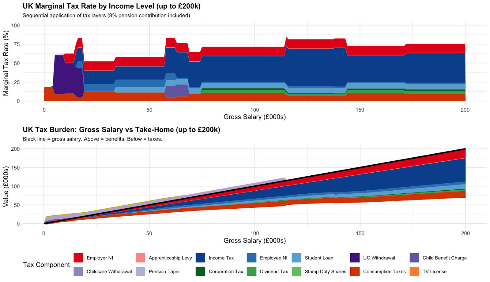
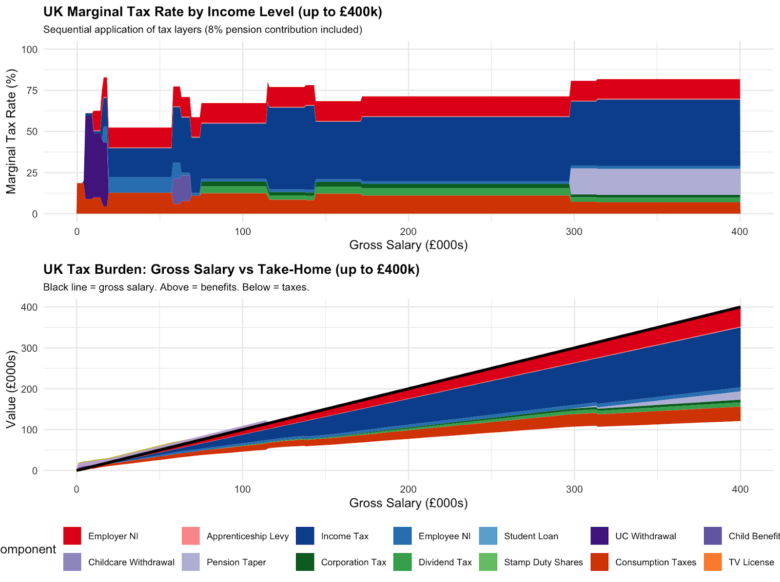
The effective rate barely differs for all realised compensations beyond £50k.
Marginal cost of public funds
Why does this matter? After all, the curve shape merely determines government revenue; for any fixed revenue requirement the curve can (and should) be made smoother by the reforms above, but why care about the overall level? Several reasons. Firstly, it would make you less optimistic about how much revenue a tax rise is likely to raise - and more optimistic about behavioural effects compensating for the costs of a tax cut.7 Secondly, it would also explain why various labour intensive sectors - such as childcare and food preparation - remain so frequently produced within households.8 There is a very large tax wedge even at the relatively low wages such workers usually earn, hence meaning that because time spent caring for children or cooking meals at home is untaxed it is routinely efficient for individuals to undertake this themselves rather than through the market.
However, we’ll here focus on the implications for cost-benefit analysis. When the government is choosing whether to make a public investment, the correct welfare criterion is not whether it generates £1 of benefit per pound spent. This is because the government can only gather the means to make investments via distortionary taxation, so activities must generate benefits over the costs of the resulting distortions.
The theoretical counterargument, advanced by Kaplow (1996, 2004) and Jacobs (2018), holds that the MCPF equals 1.0 under optimal taxation when accounting for the redistributive benefits of public spending. But even setting aside whether UK tax rates are optimal - and the proliferation of cliff edges documented above suggests they are far from it - this objection has limited force for most categories of spending subject to formal appraisal. Transport benefits are measured primarily in time savings, which scale roughly linearly with income, and more generally this is likely true for all goods the government provides without good private substitutes: willingness to pay for environmental quality, defence, or flood protection likely scales roughly linearly with income, so the equity benefits of most such schemes are minimal.
The most-cited UK estimate of the Marginal Cost of Public Funds (MCPF) is 1.26, from Kleven and Kreiner (2006), using income tax, National Insurance, and benefit tapers but not consumption or capital taxes in the marginal rate. This is representative of a literature that consistently produces values of 1.1–1.5 by applying the standard analytical formula to direct labour taxes alone, such as Browning (1987), Fullerton (1991) and Dahlby (2008). Higher estimates emerge only when the full tax system is modelled: Barrios, Pycroft and Saveyn (2013) obtained 1.81 for the UK using a CGE model that captures tax interactions of a subset of taxes endogenously, and Beaud (2011) showed analytically that incorporating VAT revenue leakage raises MCPF by 0.2–0.8 points, because reduced labour supply erodes the consumption tax base alongside the income tax base.
To estimate the Marginal Cost of Public Funds (MCPF), we take the tax rate at each income t and the elasticity of taxable income (ETI), and calculate 1 + ETI*t/(1-t). For the marginal tax rate we use the graph shown above. However, most previous estimates of the MCPF have only included direct taxes on labour when calculating this, and ignored such considerations as the income-tax-equivalent effect of benefit tapers, consumption taxes or capital levies.9 As the MCPF goes superlinearly in the tax rate, this is doubly costly.
The second key parameter for the MCPF is the elasticity of taxable income (ETI). This is because there are 3 channels that taxation could be economically costly. It could reduce hours worked per person, reduce the number of people in work or cause individuals to shift their compensation mix inefficiently - taking a job with a lower commute, for example.10 This is calculated as if compensation mix shifts are analogous to work shifts - they were entirely untaxed as is leisure. However, taxable income could also change due to redirection into corporate forms or redirection across time into lower tax periods, meaning that a pure figure for the ETI for a single revenue source is likely to be an overestimate.11
For estimates on the labour side, the total hours - combining both intensive and extensive elasticities - was estimated in Chetty et al (2013)’s meta-analysis at 0.9 leaning more heavily on micro evidence, Whalen and Reichling (2017)’s estimate for the CBO at 0.4 (range 0.27-0.53), and at 0.25 by Elminejad et al (2023).12 13 For the pure ETI, Feldstein (1999) finds 1.04 for the US in the 1980s; Browne and Phillips (2017) similarly found 0.98 under the broadest income measures from the UK’s 2010 additional rate of income tax reform, albeit under narrower specifications it can go as low as 0.35; and Gruber and Saez (2000) found an estimate of 0.4 in the US. Under the above estimates, the ETI seems very likely to at least exceed 0.4; a simple midpoint of the range would be around 0.6, and 0.8 would be possible. However, the ETI is likely higher in the US than UK on account of health insurance being such a large component of salary and lower statutory minimums for various workplace amenities providing greater margins of non-salary adjustment, and so for both these reasons and the sake of conservatism the 0.4-0.6 range will be emphasised.14
MCPF estimates also need to account for capital formation. The direct effect of taxation is to reduce labour supply, but this has a secondary consequence: with fewer effective workers, firms invest less. In standard growth models, the equilibrium capital stock is proportional to effective labour, so a 1% tax-induced reduction in hours worked leads to a corresponding 1% fall in the capital stock. This amplifies the welfare cost, and under a standard production function framework, the resulting capital reduction lowers wages by roughly 0.3%.15 The MCPF estimates presented below incorporate this adjustment as a multiplicative factor of 1.32 on the labour supply elasticity. For the purpose of calculating the MCPF given tax rates >90%, we cap the rate at 90% and pass over the excess to later incomes; this has a small impact on the results, with varying the cap from 80% to 99% only raising the estimate by 0.08 at ETI = 0.6. To ensure our worker is representative, we construct representative households on benefit-relevant characteristics from the 2023-2024 Family Resources Survey, and weight at population level frequency.
Table 1: MCPF estimates
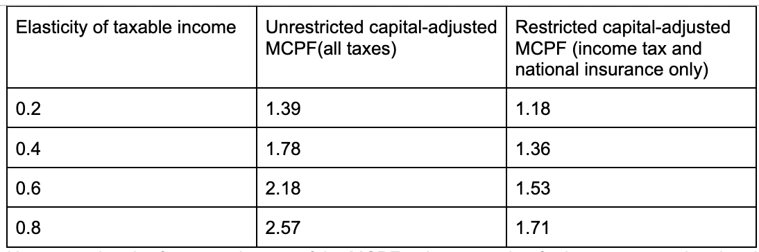
Table 2: Distribution of MCPF & deadweight loss by income bracket
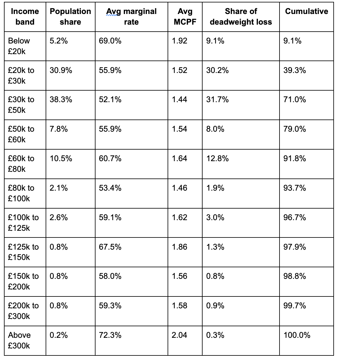
Under these elasticities, the MCPF would be ~2 in practice (unrestricted), vs ~1.4 if only income and payroll taxes were counted. This would explain the lower values common in much of the literature - as the MCPF is upward sloping in taxes, to have missed the last few components of the marginal rate would greatly reduce it. 71% of DWL comes from individuals earning below £50k, 92% from below £80k and 97% from below £125k - so this is a story of high distortionary rates affecting all workers rather than just those with high earnings.
Savings
Using data from the government’s major projects portfolio (NISTA 2024-25), there are 213 projects with total whole-life costs of £536bn. Of the 88 projects reporting monetised benefits, 69 are ongoing, representing ~£20bn in annual spending. Applying a present-value correction to whole-life costs - discounting at the Green Book rate of 3.5% assuming uniform annual spending - 64% of this expenditure has a benefit-cost ratio below 2.0 and would therefore not pass a properly calibrated cost-benefit test.16
The danger zone — projects with corrected BCRs between 1.0 and 2.0 that currently pass appraisal but would newly not automatically pass under MCPF of 2.0 — comprises 16 projects totalling £7.6bn/annum and £115bn in whole-life costs, led by the New Hospital Programme (BCR 1.26, £2.4bn/yr) (although note that this bundles the high-BCR RAAC removal that should certainly still proceed with lower-BCR new hospital construction when the return on new capital equipment for existing hospitals may be higher), the Affordable Homes Programme (BCR 1.68, £1.4bn/yr), and Smart Metering (BCR 1.35, £1.0bn/yr).17 A further 22 ongoing projects with £5.4bn in annual spending already fail at a BCR threshold of 1.0, including several major transport schemes subsequently cancelled or descoped. Infrastructure projects generally fare worst: the aggregate corrected BCR for ongoing infrastructure is just 1.30, with 77% of infrastructure spending below BCR 2.0.
These figures cover only the 5-6% of government spending that enters the GMPP and undergoes formal appraisal; the potential for savings is considerably larger if a greater share of spending were subject to cost-benefit analysis, or through implicit changes in areas such as the optimal level of subsidies and regulatory mandates.18 19 It perhaps wouldn’t be desirable to push such logic too far: the best documented parts of government are also likely the most efficient.20 However, the fact that even the most scrutinised fraction of spending contains £7.6bn of projects that would not pass a corrected cost-benefit test suggests that the true scale of mispriced public expenditure is considerably larger.
Conclusion
Marginal tax rates are frequently underestimated in policy analysis due to the need to factor in the dozens of overlapping levies, tapers and cliff edges. Beyond further raising the case for reforms to remove the largest distortions, this also implies that the threshold for public spending generating net benefits is higher than usually used. Implementing an MCPF of 2.0 in the Green Book would be an excellent opportunity for a Treasury looking to boost growth and make £8bn+ worth of savings from the expenditure judged least valuable by the departments themselves.
We refer throughout to the cost of public funds at the margin: this would of course vary if tax cuts were done in response to any savings, but the scale of appraised public expenditure is sufficiently small (at less than 2% of GDP total) for this to not much shift results.
All salaries in text will be reported post employers national insurance and the apprenticeship levy, to follow popular understanding; all salaries in graphs will be pre these to reflect costs to the employer.
VAT has a notional rate of 20%, but this has extensive exemptions for goods deemed essential, such that the tax only has an effective rate of around 12%. For a concise summary on the administrative complexity of the current system, we would direct readers to HMRC’s handy guide to the VAT rate on fur clothing. We will here assume that as a uniform VAT is distributionally neutral in the long run, consumption taxes in aggregate are. This is likely approximately correct as while VAT given exemptions is fairly progressive over the lifecycle as currently implemented (due to goods with a high income elasticity being much less likely to be zero rated, while food, housing and children’s clothing all are), other consumption taxes such as alcohol, tobacco and gambling duty are relatively regressive. Also note that we assume that all returns on savings are taxed at the UK corporation tax rate; as most OECD countries rates are higher the weighted tax for those with foreign held shares will be higher.
Here, we will assume 8% pension contributions as a share of salary, modelling the end size of pension pot and its end tax rate, which effectively lowers the marginal rate by 1-2pp.
The priority allocation for social housing is first order in many locations but will be here ignored also.
At ε=0.6, the net fiscal impact of removing each wedge is: High Income Child Benefit Charge, +£2.5bn; personal allowance taper, +£1.1bn; pension annual allowance taper, +£3.7bn; childcare cliff, −£0.6bn. The pension taper is beyond the Laffer peak at every elasticity tested, including ε=0.2, reflecting the extreme concentration of this levy on senior professionals with high scope for adjusting hours, pension contributions, and retirement timing. The childcare cliff is modelled as a binary threshold and so does not respond to the ETI framework; the true behavioural response — parents reducing hours or earnings to remain below £100k — is extensive-margin and likely larger than shown.
A caveat: these Laffer calculations assume taxpayers respond to the actual marginal rate they face. In practice, many of these wedges are poorly understood — the pension taper and childcare cliff are relatively new, and HMRC’s own research suggests many liable for the High Income Child Benefit Charge are unaware of it. The more plausible behavioural model is one in which individuals have a good sense of the broad return to work over their lifetime — informed by their overall tax burden, take-home pay, and the experience of peers — but do not finely optimise around specific thresholds they may not know exist. Under this view, the wedges are still costly (they contribute to the overall tax burden that shapes lifetime labour supply decisions) but the revenue response to removing any individual wedge would be slower and smaller than the static ETI framework implies, although their impact over general taxation may be exaggerated as non-uniform rates are more costly under the MCPF framework. The wedges are therefore more likely revenue-reducing in aggregate and over time than at the point of removal.
Which would help explain why tax-driven fiscal consolidations usually occur at much greater economic and political cost than spending-driven ones.
A similar channel explains why owner occupied housing is so much more common now than in the 19th century: the taxation of rental income but not imputed rent means that owner occupied homes bear less tax.
Many of these other taxes have other large impacts on the economy beyond their impact on individual labour supply: we ignore them here, so our estimates are a lower bound.
These are the intensive elasticity of labour supply, extensive elasticity of labour supply and the economic elasticity of taxable income.
Very high tax rates are frequently temporary in large part because they frequently raise much less money than initially anticipated due to behavioural responses (see e.g. the 2012 French and the 2010 British top rate of income tax rise).
Elminejad et al (2023) argue that earlier estimates were inflated by publication bias: however, their extensive margin elasticity is almost indistinguishable from zero, which seems highly implausible given the large variance across countries in participation rates.
We here use the uncompensated (Marshallian) elasticity, which includes both income and substitution effects, as this captures the benefit to the taxpayer of cutting taxes and then not completing the relevant project. Using compensated (Hicksian) elasticity instead implicitly assumes the project would go ahead with lump sum taxes instead of the distortionary taxes, and thus leads to slightly higher values for the MCPF as there is no effect from individuals working more in response to lower incomes, hence the fewer margins of adjustment make the change more costly for an optimising agent. We favour the uncompensated elasticity as poll taxes in practice are very rare (though occasionally used, often with dire political consequences).
Over the long run effects of taxes on emigration might be first-order relevant - the UK-US pretax income gap has averaged only 25% since 1900, comparable to the gap in disposable income additionally induced by taxation today, but UK emigration has been so large that a larger share of the descendants of people living in the UK in 1800 live in the US than UK. However, this will not be considered here as emigration occurs over much longer time horizons than most other responses to tax rates, and also emigration is fiscally ambiguous in general as it results in the loss of both tax receipts and spending obligations.
Using Gechert et al (2022)‘s estimate of 0.3 for the capital-labour elasticity of substitution, correcting for publication bias, under a CES production function.
Our PV correction assumes uniform annual spending, which likely overstates the present value of costs for infrastructure projects where expenditure follows a back-loaded S-curve — biasing our corrected BCRs downward. Working in the opposite direction, GMPP whole-life costs are reported in nominal outturn prices while benefits are in real base-year prices; correcting for the GDP deflator since each project’s base year would raise BCRs by 8–45% depending on vintage. These two biases are partially offsetting, and even if our timing assumption is off by a decade for any given project, the deflator adjustment would broadly compensate.
Specifically, the £7.6bn per year in the danger zone is dominated by five projects: the New Hospital Programme (BCR 1.26, £2.4bn/yr), the Affordable Homes Programme (BCR 1.68, £1.4bn/yr), Smart Metering (BCR 1.35, £961m/yr), Project Gigabit (BCR 1.51, £600m/yr), and the Home Office’s non-detained accommodation programme (BCR 1.23, £498m/yr). Together these account for £5.9bn of the £7.6bn total. The remainder is spread across Public Sector Decarbonisation (£480m/yr), DWP Workplace Transformation (£351m/yr), Boiler Upgrade Scheme (£199m/yr), and eight smaller programmes.
Although fitting the distribution of observed project sizes to a Generalised Pareto Distribution or other variants, even with a cutoffs to account for various different departmental reporting thresholds, suggests that there does not exist a large set of projects subject to cost benefit analysis unobserved by the central government, so there may not be much available in savings beyond the reported figure here without expanding the scope of CBR beyond its current use cases.
The economic case for rail subsidies is that there is a large fixed cost - in the form of the physical tracks and signalling system - and relatively low marginal costs. If firms had to cover this fixed cost from revenues, then they would need to set high prices relative to marginal costs - which is inefficient as there would be commuters willing to purchase trips for less than it would cost the firm to supply them, so gains from trade would be forgone. The standard solution for this is for the government to subsidise these fixed costs - which is done in the UK, with rail subsidies of £12bn/annum compared to fare revenue of £13bn. The problem is that if the government cannot raise funds lump sum, but has to acquire them through taxation, then the optimal subsidy level falls considerably.
To somewhat torture the standard metaphor, this would be a case of police ignoring other criminals to only arrest drunks under streetlights.
Thanks for this Duncan. Super interesting. I'd been about to calculate some of this myself when I was sent your piece. One comment, which may affect calculations: Employer NI is actually now at 15%, not 13.8%.
Agree. Any spending with BCR<2 is likely a net negative.
Interesting discussion about ETI. I wonder if this is why people in Asia tend to eat out more.